Data Compression

Lossy vs Lossless Compression

Back in the days of dial up modems, loading websites took a very long time. Internet speeds were slow, and it could take a minute or even longer to load webpages that required lots of images. The bigger the size of the web page, the slower it was to load, and the less likely people were to stick it out and wait.

Nowadays, broadband (including fibre optic connections) are commonplace, and pages in general load fast - even those with lots of images. However, the increased use of mobile technology has led to another problem with browsing … data limits. Pages that contain large image files, or adverts can eat away at data limits quickly, and stop people being able to access the web pages they need.

This means that we need to find ways of saving data in such a way that it takes up less space than the original file. This is called compression__. __

There are two types of compression:

1. Lossy means that data is lost and can not be recovered once the file is compressed
2. Lossless means that no data is lost and the original contents of the file can be completely recovered.

Lossy compression is useful when the specific detail of a file isn’t needed. For example, in an image, our eye may not be able to pick out the slight changes in colour in a square of 4 pixels, so by combining them into 1 single pixel (and thus decreasing the file size), it’s unlikely to make a difference.

However, lossless compression is important when all of the contents of the original file are required. For example in text documents. Your Computer Science teacher is unlikely to be particularly happy if you hand in a piece of work where half of the text is missing because the data was lost due to a lossy compression!

Run-Length Encoding (RLE)

RLE is a lossless compression technique that relies on the original piece of data having lots of repeating digits. It is about finding repeating patterns of data in a file and encoding them to save space. ‘Runs’ of data (sequences of data having the same value) are stored using frequency/data pairs.

So if we had this image:

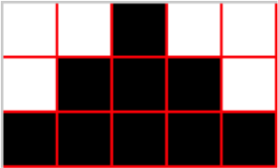
The binary code for this is 0010 0011 1011 111. We now want to instead write it as a ‘say what you see’ sequence. So instead we have 2 zeros, 1 one, 3 zeros, 3 ones, 1 zero, 5 ones, which in run-length encoding would be:

(2 0), (1 1), (3 0), (3 1), (1 0), (5 1)

The first value in each pair is the frequency (how many there are) and the second is the data (the actual number).

Compress these using RLE. Don't leave a space or any other punctuation between each value.1 1 1 1 1 1 0 0 0 0 1 1 1 1 1 1 0 0 0 0

1525708078122

Compress these using RLE. Don't leave a space or any other punctuation between each value.0 0 0 1 1 1 1 0 0 1 0 0 1 1 1 0 0 1 0 1

30412011203120111011

Decompress these using RLE. Don't leave any spaces.(3 1), (3 0), (3 1), (3 0), (1 1), (1 0), (1 1), (1 0), (1 1), (1 0), (3 1), (3 0), (3 1), (3 0)

111000111000101010111000111000

Decompress these using RLE. Don't leave any spaces.(7 1), (3 0), (3 1), (3 0), (4 1)

11111110001110001111

Huffman Encoding

This is another lossless data compression model that makes use of the frequency of characters in a string.

For example, the string “a ratty character” has quite a lot of repeated letters in it. In fact, it only contains 8 different characters - “a rtyche” (Note the space is important here!).

Now if we were to store this using 7-bit ASCII, this string would require 119 bits (17 * 7). Using RLE here would be useless, as there is only 1 substring that contains any repetition, so we need to find a new way of doing it…

There are two parts when using Huffman’s technique:

1. A Huffman tree – this gives each character used a unique code.
2. Binary stream of the character sequence

This is how we generate both for the example “a ratty character”.

Creating the Huffman Tree

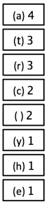
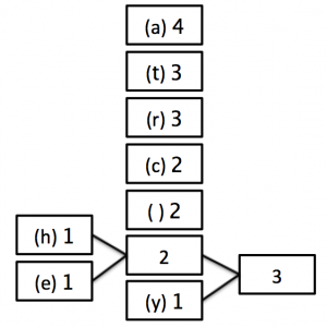
1) Count how many times each character appears in the sentence and write the list so that the highest frequency letter appears at the top.

2) Now, combine the two lowest occurring numbers together into one block and label it with the added frequency of those two blocks.

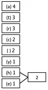
3) Now, move the new block that you have created (and any blocks attached to it) into position in the list of numbers - if there is more than 1 value the same, it doesn’t matter which order you choose.

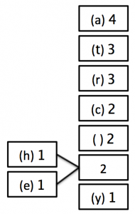
4) Keep repeating steps 2 and 3 until there is only 1 block remaining as follows:

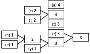
STEP 2:

STEP 3:

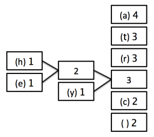
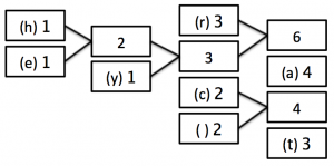
STEP 2:

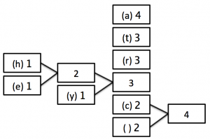
STEP 3:

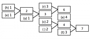
STEP 2:

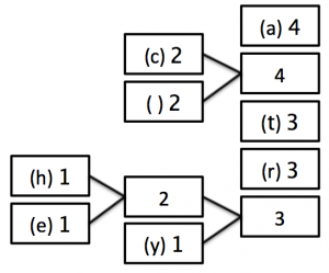
STEP 3:

STEP 2:

STEP 3:

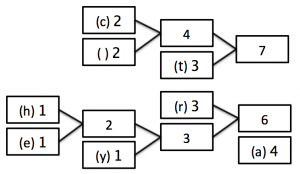
STEP 2:

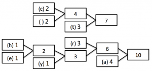
STEP 3 - Finished position:

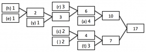
In this last tree, you can see that we are now left with only one box (called a ‘node’) which has a frequency of 17 - the number of characters in our string!

4) Now we have our tree, it’s time to label the branches. You may come across instances where you aren’t required to label the branches, but you will instead be given a specific code which will allow you to work out what the labels should be. To avoid making mistakes, it is worth adding the labels.

Working from the single node, label all up arrows 1, and all down arrows 0 (or vice versa - but be consistent!)

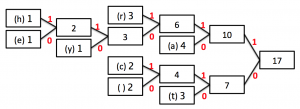
This is our finished Huffman tree!

Encoding the Binary Stream

Now we have our tree, it’s time to actually compress our string. Remember, we are trying to compress “a ratty character” down from the 119 bits that would be required to store it using ASCII.

To create the string, first we need to know how to ‘read’ a Huffman tree. To do this, you start at the single ‘big’ node - in our case 17. Then each letter is encoded using the path of 1s and 0s from there.

For example, the letter “a” is now encoded as 10, whilst the stream 11010 is decoded to the character ‘e’. Notice that the letters with the greatest frequency now have the shortest binary representation. This is our trick to reducing the storage requirements of the string.

Getting back to the Binary stream, we now go through letter by letter and work out what the binary representation is for each one:

1. a: 10
2. t: 00
3. r: 111
4. c: 011
5. SPACE: 010
6. y: 1100
7. h: 11011
8. e: 11010

Then we go back to our original string and join them together:

“a ratty character” becomes 10 010 111 10 00 00 1100 010 011 11011 10 111 10 011 111 11010 111

This is now a measly 50 bits in comparison to the original 119 required!

In reality, Huffman encoding wouldn’t be as good as this, as the Huffman tree would also need to be sent along with the binary stream, which will take up additional bits. However, in the exam, you may be asked to calculate how many bits are stored by doing a Huffman compression of a piece of text vs using ASCII.