Price Elasticity of Supply

Price Elasticity of Supply (PES) measures the responsiveness or sensitivity of supply to changes in price. It is calculated as follows:

PES = %Change in Quantity Supplied ÷ %Change in Price

This can be broken down into the following:

%ΔQS = [(Q2-Q1) ÷ Q1] X 100 ÷ %ΔP = [(P2-P1) ÷ P1] X 100

Q1 = original quantity, Q2 = new quantity, P1 = original price, P2 = new price

Example

The price of petrol increases from £1.00 to £1.30 per litre. As a result supply expands from 10 million to 11 million litres per day. Calculate the PES of petrol, using the formula:

PES = %ΔQS ÷ %ΔP

Workings:

Q1 = 10m, Q2 = 11m, P1 = £1.00, P2 = £1.30

Firstly, calculate the % change in quantity supplied:

%ΔQS = [(11-10) ÷10] X 100

= (1 ÷ 10) X 100

= 0.1 X 100

= 10%

Now calculate the % change in price:

%ΔP = [(1.3 -1.00) ÷ 1.00] X 100

= (0.3 ÷ 1.00) X 100

= 0.3 X 100

= 30%

Finally, PES = %ΔQS ÷ %ΔP = 10 ÷ 30

Answer: PES = 0.3

Note that PES is always a positive value. This is because the change in price and quantity are either both positive or both negative. If price goes up, quantity supplied goes up; if price goes down, quantity supplied goes down too.

Note also that there are no ‘units of elasticity’. The value 0.3 simply means that supply has changed proportionately only 0.3 (or 30%) as much as price. PES is really a ratio.

In this case the value of PES is less than 1 or unity. This is called inelastic demand___. ___This means supply changes proportionately less than price.

Summary Table of PES

Numerical Value of PES	Term	Description
0 or Zero	Perfectly inelastic	Quantity supplied is unchanged when price changes
Between 0 and 1	Inelastic	Quantity supplied changes by a smaller % than price
1 or Unity	Unit elasticity	Quantity supplied changes by the same % as the change in price.
Between 1 and Infinity	Elastic	Quantity supplied changes by a greater % than the change in price
Infinity	Perfectly or infinitely elastic	Quantity supplied is zero at any lower price, but unlimited at a given price.

Some Special Cases

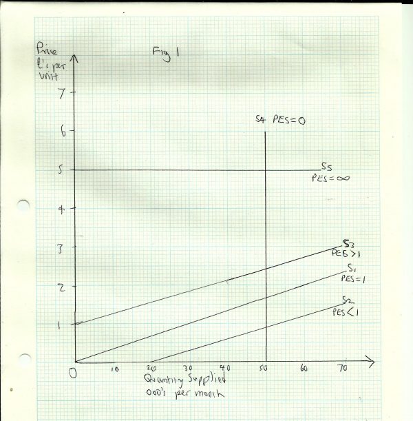
In Fig 1 any straight line supply curve, such as S1 that passes through the origin, has a constant PES = 1. This will be true regardless of the gradient. For instance, if price doubles from £1 to £2, quantity supplied also doubles, from 30,000 to 60,000 per month.

Any straight line supply curve, such as S2 that passes through the quantity axis has a PES < 1, since the quantity supplied changes by a smaller % than the change in price.

Any straight line supply curve, such as S3 that passes through the price axis has a PES > 1, since the quantity supplied changes by a greater % than the change in price.

Note that S1, S2 and S3 all have the same gradient, but different values for PES. The actual change in quantity supplied for any given change in price is the same in all three cases; a rise in price of £1 per unit results in an expansion of supply of 30,000 units. But in each case, the proportionate change in quantity is different, because the original quantity is different in each case.

Supply curve S4 is a vertical straight line, which means that the quantity supplied is the same at all prices, so PES = 0. This is only likely to apply in the very short term, in a situation where producers cannot yet respond to a change in price by raising output.

S5 __is a horizontal straight line, where __PES = infinity. At any price below £5 per unit, quantity supplied is zero, but at £5 it is unlimited. This only arises under conditions of a perfectly competitive market. A small dairy farmer, for instance, can buy as much straw for his cattle as he needs at the market price, because he represents only a tiny fraction of total demand.

Factors Determining PES

Time period - It takes time for producers to adjust output to changes in price; they need to acquire more (or fewer) factors of production. In capital intensive industries, such as electricity generation it can take several years to install a new power station. In the short run supply will be less elastic than in the long run
__Mobility of factors of production __- Some industries use resources which have no alternative use. For instance a coal mine can only produce coal, so supply is likely to be relatively inelastic. But a factory that currently makes petrol fuelled cars could fairly quickly change to producing electric powered vehicles. So if the price of the former falls, supply is likely to be relatively elastic, as producers switch to making something more profitable
__Capacity utilisation __- If a firm or an industry is currently operating close to its maximum capacity, it cannot easily raise output when price rises, so supply will be relatively inelastic. Where there is spare (unused) capacity, supply is more elastic
Stock levels -In some industries it is possible to supply the market from stocks of goods made earlier. For instance, meat can be stockpiled in refrigerated warehouses. But most services have to be produced at the moment they are wanted (i.e. hairdressing). Where stocks can be maintained, supply is relatively elastic
__Ease of entry to the market __- Where it is easy for firms to enter or leave the market, supply will be relatively elastic and vice versa