The Multiplier
The Multiplier
The multiplier __is a ratio that determines how much national income (__Y) will change if there is an increase or decrease in any of the injections (J) - [investment (I), government spending (G) or exports (X)].
To understand the multiplier, consider the following simple example:
Suppose a firm spends £10m to build a new factory. (in other words I increases by £10m). Assume also that there is no foreign trade (imports or exports) and no public sector (government spending and taxation. But, households always save 10% (0.1) of any increase in their income.
The investment spending (£10m) becomes income to the workers, managers and owners of the construction company building the factory.So national income (Y) has risen by £10m.

But this is not the end of the process. The workers, managers and owners will now spend £9m and save £1m (assuming they save 10%).
This £9m of spending becomes income to the shopkeepers, restaurants etc where it is spent. So Y has risen by a further £9m.
Of this £9m, another £8.1m gets passed on as spending and £0.9m will be saved.
At this point we can see that income has now risen by £10m + £9m + £8.1m = £27.1m
There will continue to be further rounds of spending and saving, each one smaller than the last.
We can calculate the final change in national income (ΔY) resulting from this initial change in an injection (ΔJ) by firstly working out the value of the multiplier (K):
K__ = __1/1-mpc, where mpc = marginal propensity to consume.
In this case __mpc __= 0.9 - This is because households save 0.1 of any increase in income and therefore must spend the remainder (we have assumed no income is taken in tax or spent on imports).
Therefore: K = 1 / 1-0.9 = 1 / 0.1 = 10
The final change in national income is now calculated using the formula:
Δ Y = Δ J X K
= £10m X 10
= £100m
In this case therefore, the initial increase in investment has resulted in a final increase in income 10 times larger.
A More Realistic Multiplier
In the real world, the value of the multiplier is much smaller. This is because some part of any increase in income is withdrawn from the circular flow in taxation (T) or imports (M).

Let’s reconsider the example above, but this time we will assume the following:
Households save 10% of any increase in income: the marginal propensity to save (mps) = 0.1
25% of any increase in income is taken in tax: __the marginal rate of tax (mrt) __= 0.25
20% of any increase in income is spent on imports: __the marginal propensity to import (mpm) __= 0.2
The sum of the (mps + mrt + mpm) is called the marginal propensity to withdraw(mpw).
In this case it is 0.55 (0.1 + 0.25 + 0.2).
We can now calculate the multiplier using the formula:
K__ = 1/mpw = __1/0.55 = 1.82 (to 2 dec places)
Going back to our example, the final change in income will now be:
£10m X 1.82 = £18.2m
This is a much more realistic figure. In the real world the value of the multiplier is likely to be somewhere between 1.5 and 2.
Positive and Negative Multiplier Effects
The larger change in Y compared to the change in J __is called the multiplier effect__. In our example it is a positive effect, because J, and therefore__ Y have both increased. But if investment had fallen, the multiplier effect would have been negative, and the fall in __Y __would be greater than the fall in J__.
Changes in the Value of the Multiplier
mpc + mpw = 1
It therefore follows that the value of __K __depends on the size of the mpw (or equally the mpc). The greater the mpw (or the smaller the mpc), the smaller will be the value of the multiplier.
It also follows that any change in the size of the components of mpw (mps, mrt or mpm) will affect the value of the multiplier.
Going back to our example above, let us suppose that the mpm falls from 0.2 to 0.15. The mpw will now be: [mps (0.1) + mrt (0.25) + mpm (0.15)] = 0.5
So the value of the multiplier (K) is now 1/0.5 = 2.0
This means the final change in national income resulting from the £10m would now be £20m rather than £18.2m.
NB: You should think about how changes in the economy may affect mpc, mps, mrt or mpm. For instance, a rise in the exchange rate will make imports more competitive, leading to an increase in mpm and therefore a fall in the value of the multiplier.
How the Multiplier Affects AD and Equilibrium Output
As we have seen, the multiplier effect means that the final increase in _Y __is greater than the initial change in injections. This is shown in _Fig 1 below:
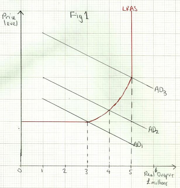
The initial equilibrium level of __Y __is £3bn. Suppose the value of the multiplier is 2 and there is an increase in investment of £1bn. This will shift AD from AD1 to AD2, and __Y __will increase by £1bn, from £3bn to £4bn.
But this is not the end of the process. The multiplier effect means that the investment spending gets passed on in the circular flow, as we have seen. The final equilibrium will be £5bn, and AD will have shifted further, to AD3 as additional spending takes place. A fall in investment would have the opposite effect, pushing AD back to the left, and the fall in Y would be greater than the fall in investment.
The Multiplier and Managing the Economy
The precise value of the multiplier is unknown, although governments and forecasting bodies do their best to estimate it from known economic data on changes in spending and national income in the recent past. However, as we have seen, the variables that determine the value of the multiplier are constantly changing, so data from recent months or years will not give us certainty over its value in the future.
Governments would like to know its value, as this has implications for how it manages the economy, especially when using fiscal or monetary policies to try to stimulate or slow down the economy_._ For instance, if the government wants to raise Y __by £10bn, it could be achieved with an increase in government spending (__G) of £5bn if the multiplier is 2. But if the multiplier was 1.5 an increase in __G __of £6.7bn would be needed.