Equilibrium Levels of Real National Output
Equilibrium Levels of Real National Output
The economy is in macro-economic equilibrium when aggregate demand (AD) equals aggregate supply (AS). We can distinguish between short and long run equilibrium.
Short Run Equilibrium
This occurs when AD = SRAS. This is shown in Fig 1 below:
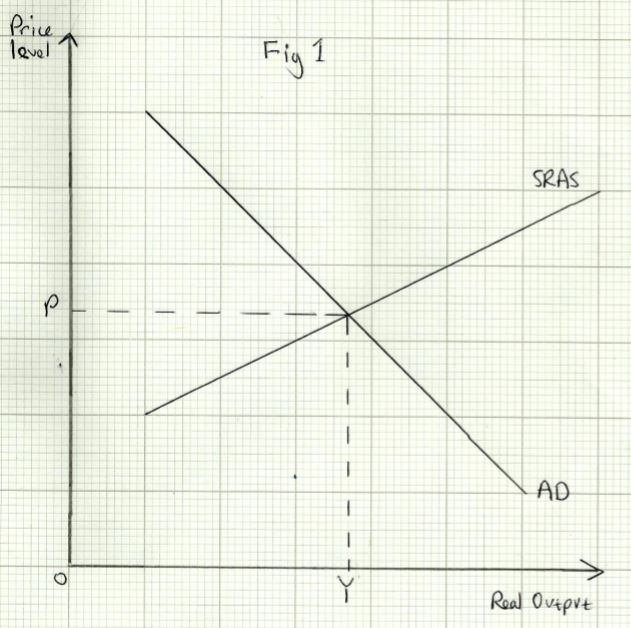
The economy is in short run equilibrium at a price level of P __and real national output of __Y. The level of AD [C+I+G+(X-M)] is just equal to the value of firms’ output.
Shifts in AD
An increase or decrease in AD will cause a change in short run equilibrium, as shown in _Fig 2 _below:
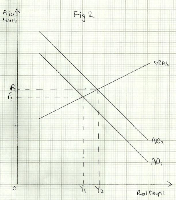
An increase in AD could come about in a number of ways, for example a fall in interest rates which would encourage investment and consumption. This is shown by an outward shift from AD1 to AD2 on the diagram. This results in both an increase in real output (from Y1 to Y2 and a rise in the price level (from P1 __to __P2). A decrease in AD from AD1 to AD2 will cause real output and the price level to fall.
An increase or decrease in SRAS will also cause a change in short run equilibrium, as shown in _Fig 3 _below:
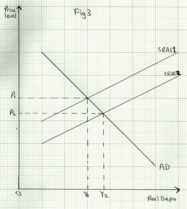
An increase in SRAS is shown by the move from SRAS1 to SRAS2. This could come about for a number of reasons. For instance, there may be a fall in imported raw materials prices.
The increase in SRAS results in both a fall in the price level (from P1 to P2) and an increase in real output (from Y1 to Y2). A decrease in SRAS will cause real output to fall and the price level to rise.
Long Run Equilibrium
Neo-classical and Keynesian economists agree on the nature of short run equilibrium, but are divided in their approach to long run equilibrium, because of their differences on the nature of long run aggregate supply.
Neo-Classical View of Long Run Equilibrium
To be in long run equilibrium, not only must AD = LRAS, but also SRAS. This is shown in _Fig 4 _below:
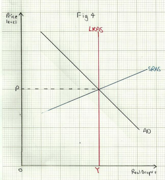
The economy is in both short and long run equilibrium at a price level P and a level of real output at__ Y__, where the economy is at full employment, which neo-classical economists regard as the normal state of affairs.
Now let’s consider what happens if there are changes, in AD, SRAS, or LRAS according to the neo-classical view.
Change in AD
A change in AD is shown in Fig 5, below:
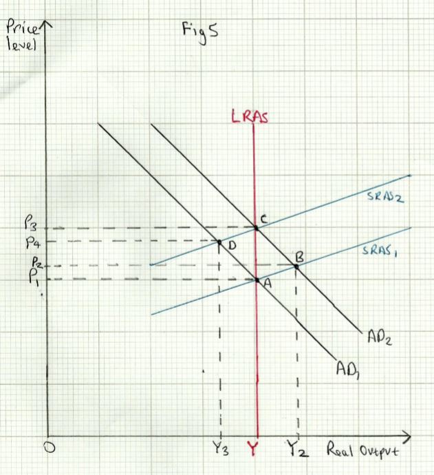
The economy is initially in equilibrium at point A __(AD = SRAS = LRAS). Let us suppose that there is an increase in AD, so that there is a new short term equilibrium at point __B, where AD2 = SRAS.
Real output and the price level will rise to Y2 __and P2__ respectively.
But this is not a stable equilibrium_. _The economy has a positive output gapmeaning it is operating beyond its sustainable level of output. The rise in the price level to P2 will reduce workers real wages, even though money wages haven’t changed. Eventually, as workers realise this, they will bargain for higher wages, and will probably expect further price rises, so they will seek a big enough pay rise to protect themselves from anticipated inflation.
This results in a shift of short run aggregate supply from SRAS1 to SRAS2. Equilbrium moves to point C. Note that real output is back at Y __(the full employment level), but the price level has now moved up to __P3.
A decrease in AD can be explained by assuming the economy is initially at point C. If AD decreases, it moves from AD2 to AD1. The economy is now in a new short run equilibrium at point D. The price level and real output have fallen to P4 __and __Y3 respectively. The economy is now operating below capacity (negative output gap) and there is some unemployment.
The fall in the price level means that real wages have risen. Together with the fact that workers have less bargaining power due to the rise in unemployment, wages should fall. This results in a downward shift of short run aggregate supply to SRAS1. The economy is now in long run equilibrium again at full employment at point A, and there has been a further fall in the price level to P1.
Change in LRAS
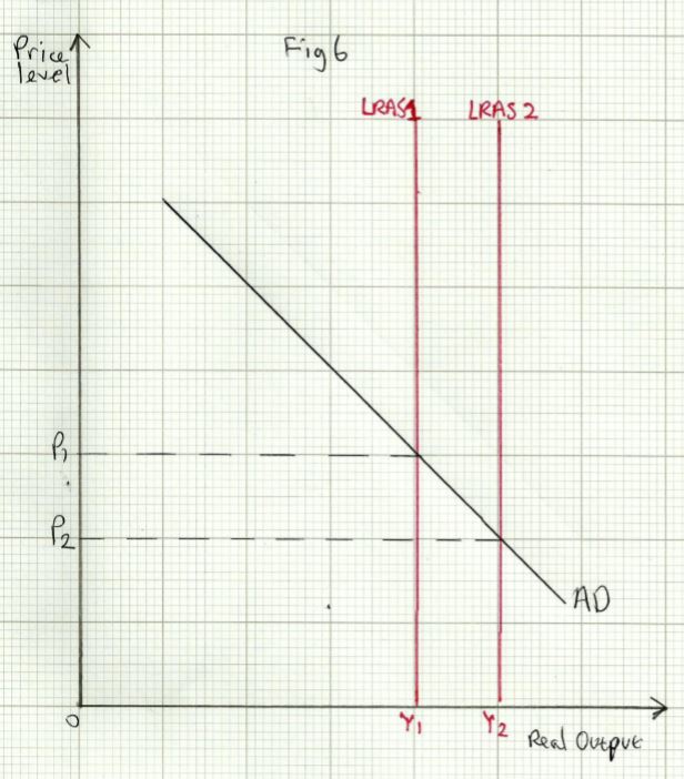
An increase in LRAS is represented by an outward shift from LRAS1 to LRAS2. This can happen for a number of reasons_. _This results in an increase in real output (from Y1 to Y2) and a fall in the price level (from P1 to P2). Neo-classical economists believe that policies to increase LRAS are the best way to ensure sustainable growth in the economy, as it does not lead to higher inflation.
By contrast, they argue that policies to promote growth by boosting AD only lead to a temporary increase in output, but also create more inflation (higher prices). This is shown in Fig 5.
It is possible that LRAS can decrease, in which case real output will be lower and prices will be higher.
The Keynesian View of Long Run Equilibrium
The Keynesian LRAS is perfectly elastic at low levels of output, and becomes perfectly inelastic at full employment_. _Keynesian economists argue that it is quite possible for the economy to be in long run equilibrium at an output below full employment. The reject the view that the economy automatically returns to full employment. The main reason for this is that wages cannot easily adjust downwards in a recession.
There are number of reasons for this:
- Trade unions will resist pay cuts, so there may be industrial disputes
- Minimum wage laws prevent falls in wages below the legal minimum
- Out of work benefits may make low paid jobs unattractive
Change in AD
The Keynesian view of a change in AD on long run equilibrium is shown in Fig 7 below:
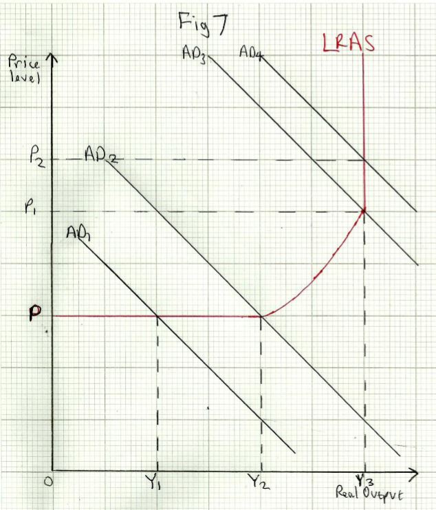
When aggregate demand is at AD1, there is high unemployment, with real output at Y1 __and the price level at P__. If Aggregate demand increases to AD2, real output rises to Y2 without any increase in the price level. This is because there is still substantial spare capacity in the economy. Workers will not yet have bargaining power to drive up wages.
Any increase in AD between AD2 and AD3 will result in an increase in real output, but the price level will also rise, as shortages of labour and other inputs start to drive up costs.
At AD3 the economy is in full employment at a level of real output and prices of Y3 __and __P1 __respectively. Any further increase in AD (i.e. to AD4), will not result in a long term increase in output, just higher prices at __P2. In other words, at full employment. Keynesians and neo-classical economists are in agreement; LRAS is vertical.
Change in LRAS
A shift in LRAS is shown in Fig 8 below:
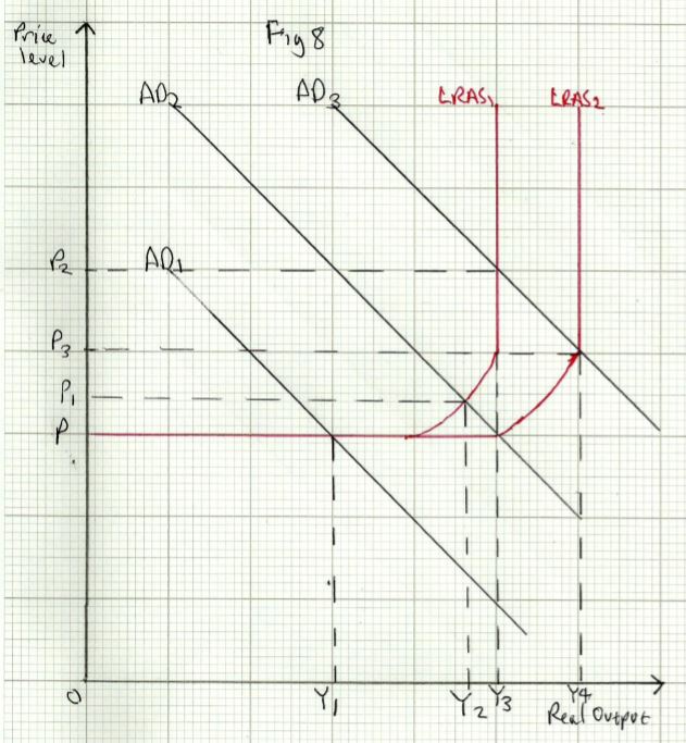
The effect of an increase or decrease in LRAS on equilibrium output and prices depends on the level of AD. If aggregate demand is at AD1, an increase in long run aggregate supply from LRAS1 to LRAS2 will have no effect on output or prices.
At AD2, however there will be an increase in real output (from Y2 to Y3) and the price level will fall (from P1 __to __P). This is because the increase in LRAS has increased the capacity of the economy and eased shortages of labour and other inputs, creating downward pressure on prices.
If the economy was already at full employment, with AD at AD3, the increase in LRAS will also result in higher output and lower prices ( Y4 and P3, rather than Y3 and P2).
A decrease in LRAS would result in higher prices and lower output, unless AD was already weak (as at AD1), in which case prices and output would be unchanged.
Investment: the Link Between AD and LRAS
It is of course possible that both AD and LRAS change over time. The most likely reason for this is a change in investment spending.
Investment is both a component of AD and is a critical factor in determining the level of productive capacity and long term growth in the economy. Fig 9 below shows the impact of higher investment on the economy:
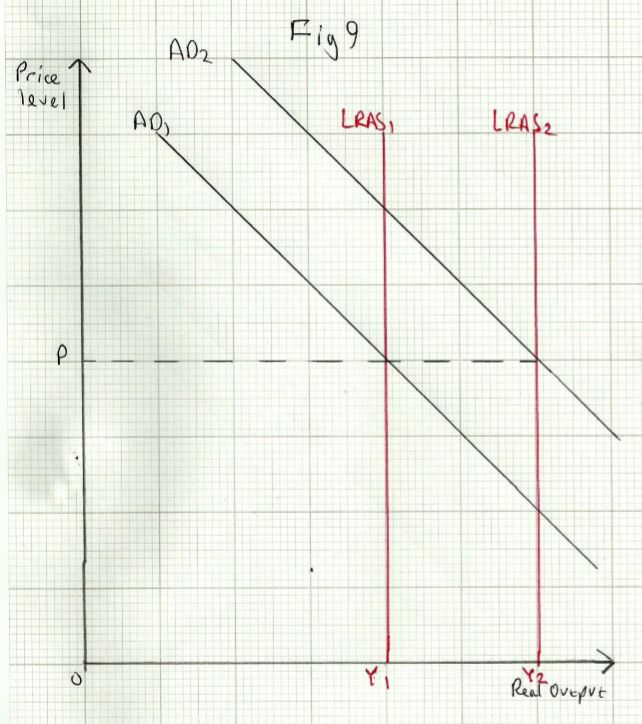
The increased investment increases AD from AD1 to AD2, and LRAS increases from LRAS1 to LRAS2. This results in higher real output at Y2. The diagram shows the price level P, to be unchanged. But this depends on the extent to which AD increases and LRAS increases. It is possible that the price level could be higher or lower than P.
This will depend on a number of factors such as:
- The amount spent on the investment (the more spending, the greater the increase in AD)
- The productivity of the investment (the extent to which does it actually raise capacity)
- The time taken for the investment spending to become operational (for instance the spending on HS2 high speed rail won’t see any trains running until 2032).