Price, Income & Cross Elasticities of Demand

Price Elasticity of Demand (PED)

PED measures the responsiveness or sensitivity of demand to changes in price. It is calculated as follows:

PED = % Change in Quantity Demanded ÷ % Change in Price

This can be broken down into the following:

%ΔQD = [(Q2-Q1) ÷ Q1] X 100 ÷ %ΔP = [(P2-P1) ÷ P1] X 100

Q1 = original quantity, Q2 = new quantity, P1 = original price, P2 = new price

Example 1

The price of petrol increases from £1.00 to £1.30 per litre. As a result demand contracts from 10 million to 9 million litres per day. Calculate the PED of petrol, using the formula:

PED = %ΔQD ÷ %ΔP

Workings:

Q1 = 10m, Q2 = 9m, P1 = £1.00, P2 = £1.30

Firstly, calculate the %__ change in quantity demanded:__

%ΔQD = [(9-10) ÷10] X 100

= (-1 ÷ 10) X 100

= -0.1 X 100

= -10%

Now calculate the %__ change in price:__

%ΔP = [(1.3 -1.00) ÷ 1.00] X 10

= (0.3 ÷ 1.00) X 100

=0.3 X 100

= 30%

Finally, PED = % ΔQD ÷ %ΔP

=-10 ÷ 30

Answer: PED = -0.3

Note that PED is always a negative value. This is because we are dividing a negative value by a positive value, or vice versa. In other words if price goes up, quantity demanded goes down, or vice versa.

Note also that there are no ‘units of elasticity’. The value 0.3 simply means that demand has changed proportionately only 0.3 (or 30%) as much as price. PED is really a ratio. In this case the value of PED is less than -1 or unity. This is called _inelastic demand. ___This means demand changes proportionately less than price.

Example 2

Following a cut in airline ticket prices from London to New York from £1000 to £850, sales of tickets rise from 1200 to 1500 per week. Calculate the PED of airline tickets.

Workings:

Q1 =1200, Q2 = 1500, P1 = £1000, P2 = £850

Firstly, calculate the %__ change in quantity demanded:__

% ΔQD = [(1500-1200) ÷ 1200] X 100

= (300 ÷ 1200) X 100

= 0.25 X 100

= 25%

Now calculate the %__ change in price:__

%ΔP = [(850 -1000) ÷ 1000] X 100

= (-150 ÷ 1000) X 100

= -0.15 X 100

= -15%

Finally, PED = %ΔQD ÷ %ΔP

= 25 ÷-15

Answer: PED = -1.67

Note that this time the value of PED is greater than -1. This is called elastic demand. This means demand changes proportionately more than price.

Cross Elasticity of Demand (XED)

XED measures the responsiveness of demand of one good to a change in the price of another good.

XED = % Change in Quantity Demanded (of Good A) ÷ % Change in Price (of Good B)

This can be broken down into the following:

%ΔQDA = [(Q2-Q1) ÷ Q1] X 100 ÷ %ΔPB = [(P2-P1) ÷ P1] X 100

Q1 = original quantity (of good A), Q2 = new quantity (of good A), P1 = original price (of good B), P2 = new price (of good B)

Example

The price of a computer games console (Good B) falls from £500 to £400. As a result sales of games (Good A) increase from 50,000 to 70,000 per month. Calculate the XED of computer games with respect to the price of consoles.

Workings:

Q1 = 50,000, Q2 = 70,000, P1 = £500, P2 = £400

Firstly, calculate the % change in quantity demanded for Good A:

% ΔQDA = [(70,000-50,000) ÷ 50,000] X 100

= (20,000 ÷ 50,000) X 100

= 0.40 X 100

= 40%

Now calculate the % change in price of Good B:

%ΔP = [(500 - 400) ÷ 500] X 100

= (-100 ÷ 5 00) X 100

= -0.20 X 100

= -20%

Finally, XED = %ΔQDA ÷ %ΔPB

= 40 ÷ -20

Answer: XED = - 2.0

Games consoles and the games that run on them is an example of complementary or joint demand. We use the two goods together. These goods have a negative XED. Firms can use this relationship to their advantage. For instance, computer printers are generally very cheap, generating sales of ink cartridges which tend to be expensive. The printer manufacturer makes most of their profit on the ink cartridges.

For goods like bread and butter, the relationship between them is not so strong; we don’t always consume them together so the value of XED is likely to be much lower, between 0 and -1.

XED is also important in the case of _substitute goods. ___These are goods that satisfy the same need. For instance, we can use margarine instead of butter, or drink a different brand of cola. Goods which are substitutes for each other will have a __positive XED, __since a rise in price of Good B will result in an increase in demand for good A (the substitute).

Where goods are very close substitutes, such as alternative suppliers of electricity or different phone networks the XED is likely to be greater than +1, for goods that are not close substitutes such as beer and wine, the value of XED is likely to be between 0 and +1.

Zero, Infinity and Unity

Three Special Cases of Price Elasticity of Demand: Zero, Infinity and Unity

Fig 2 below shows three special cases of elasticity:

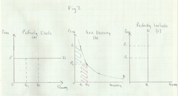
In (a), demand is perfectly elastic, represented by a horizontal straight line. At any price above P, there is no demand, but at price P, the producers can sell everything they are able to, for instance Q1 or Q2. This is a feature of Perfect Competition.

Diagram (b) __shows __unit elasticity, which means that any % change in price is offset by an equal and opposite % change in quantity, so total spending remains unchanged. For instance, if price falls from P1 to P2, quantity increases from Q1 to Q2. The green area represents a fall in spending that is equal to the red area, which represents an increase in spending.

In (c), demand is perfectly inelastic. This means that the quantity demanded is the same at all prices, such as P1 or P2. Total spending is therefore directly proportional to price; if price increased by 50%, spending would also increase by 50%.

Summary of Price Elasticity of Demand

Measure of PED	Term	Description	Effect on Spending of Price Rise	Effect on Spending of Price Fall
Infinity	Perfectly elastic	Quantity demanded is unlimited at a given price, but zero demand above this price	Falls to zero	Falls by the same % as price
Greater than -1	Elastic	Quantity demanded changes by a larger % than does price	Decrease	Increase
-1	Unitary elasticity	Quantity demanded changes by the same % as does price	No change	No change
Between 0 and -1	Inelastic	Quantity demanded changes by a smaller % than does price	Increase	Decrease
0	Perfectly inelastic	Quantity demanded is the same at all prices	Increases by the same % as price	Falls by the same % as price.

Factors affecting price elasticity of demand:

1. Marketing and branding - Successful marketing, including advertising can create strong brand loyalty amongst consumers. This reduces PED and gives the producer greater ability to raise price
2. __Availability of substitutes __- If there are plenty of alternatives to the good in question, demand is likely to be more elastic
3. How widely the market is defined - The demand for a particular kind of soft drink, such as cola, will be more elastic than the demand for soft drinks as a whole, which includes lemonade and fruit juice
4. Proportion of income spent on the good - A 20% increase in the price of petrol would probably result in a bigger reduction in petrol consumption compared to the reduction of salt consumption if its price increased by 20%. This is because the former will have a much greater impact on the household budget
5. __Time period __– The demand for any good is likely to be more elastic in the long term compared to the short term. This is because we can more easily adjust our consumption over time. A big rise in gas prices might not have much impact on demand in the short run, but over time people will invest in insulation and switch to other means of heating and cooking
6. __Is the good a necessity or luxury __- Goods or services which are thought of as essential tend to have a lower PED than those which we think we can go without if they are expensive

Income Elasticity of Demand (YED)

YED measures the responsiveness of demand to changes in people’s incomes. It is calculated as follows:

YED = % Change in Quantity Demanded ÷ % Change in Income

This can be broken down into the following:

%ΔQD = [(Q2-Q1) ÷ Q1] X 100 ÷ %ΔY = [(Y2-Y1) ÷ Y1] X 100

Q1 = original quantity, Q2 = new quantity, Y1 = original income, Y2 = new income

Example

After a pay rise, Tracey’s wage rises from £200 to £230 per week. She finds she can afford to go out more, so her weekly consumption at the nearby wine bar goes up from 6 to 10 glasses per week. Calculate Tracey’s YED for wine.

Workings:

Q1 =6, Q2 = 10, Y1 = £200, P2 = £230

Firstly, calculate the % change in quantity demanded:

%ΔQD = [(10-6) ÷ 6] X 100

= (4 ÷ 6) X 100

= 0.67 X 100

= 67%

Now calculate the % change in income:

%ΔY = [(230-200) ÷ 200] X 100

= ( 30÷ 200) X 100

= 0.15 X 100

= 15%

Finally, PED = % ΔQD ÷ %ΔY

= 67 ÷ 15

Answer: YED = 4.47

In this case the YED is a positive value, since quantity demanded has increased as a result of an increase in income (and would fall if income fell). Goods with a positive YED are called __normal goods __and account for the large majority of goods.

In this case, the YED > 1, so demand is income elastic, meaning that demand changes by a greater proportion than income. Goods with high positive values for YED (greater than +1) are sometimes called luxury goods. The sale of such goods and services will tend to do well when the economy is growing fast and incomes are rising. In a recession, they are likely to fall quite rapidly.

Goods where YED<1 __are called __necessities_._ Suppose for instance that the sale of toothpaste fell by 1% following a fall in incomes of 10%. The value of YED in this case would be +0.1. In this case demand is income inelastic. It is a positive value because the change in income and demand are both negative (or positive if income rises). Demand for necessities tends to be more stable, and fluctuates less with changes in income.

There is a special class of goods that has a negative YED. These goods are called inferior goods_._

These are goods or services we tend to buy less of as our income rises. For instance, bus travel in Britain has been falling for many years as more people have cars. Suppose that bus travel falls by 1% for every 5% increase in average incomes. The YED would be -0.2. it is negative because the change in demand is negative when the change in income is positive (and vice versa).

Price Elasticity of Demand and Total Spending

Consider again the data in Examples 1 & 2, and how total spending changes when price changes.

In Example 1, total spending (price X quantity) increases from £10 m to £11.7 m when price rises from £1.00 to £1.30. It follows that a fall in price from £1.30 to £1.00 would cause total spending to fall from £11.7 million to £10 million.

When demand is price inelastic, a rise in price results in an increase in spending and vice versa.

In Example 2, a fall in price from £1000 to £850 results in an increase in spending from £1.2m to £1.275m, and vice versa.

When demand is price elastic, a rise in price results in a decrease in spending and vice versa.

The relationship between spending and price elasticity of demand is shown in _Fig 1 _below:

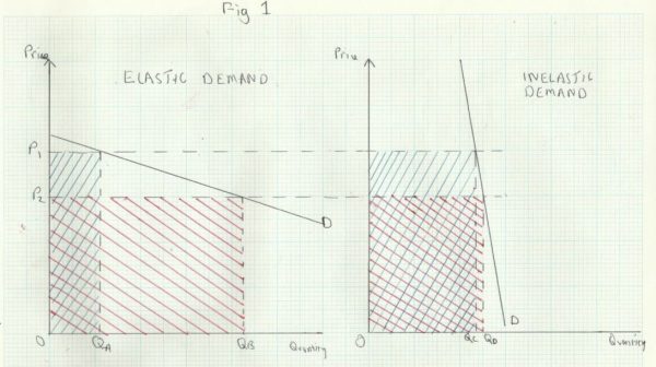
The diagram on the left shows that demand is price elastic between prices P1 and P2. The green shaded area represents total spending at P1 and the red shaded area shows spending at P2. Spending rises when price falls and vice versa.

The opposite situation is shown on the right hand diagram, where demand is price inelastic the fall in price from P1 to P2 results in a fall in spending and vice versa.