Aggregate Supply

Short Run Aggregate Supply

__Aggregate supply __refers to the value of the total output of goods and services in the economy in a given period of time, at any given price level. We can distinguish between short run aggregate supply (SRAS) and long run aggregate supply (LRAS).

Short Run Aggregate Supply

The ‘short run’ in this context means that factor prices (wages, interest and rents) do not change. This is often taken to be a period of less than a year, as most wages and other actor costs are usually negotiated annually.

The SRAS curve is upward sloping, as shown in Fig 1 below:

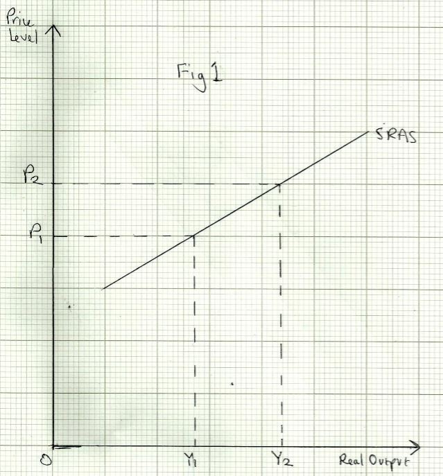
Just as with the supply of any particular good, if firms in general increase output, the marginal cost of additional units produced tends to increase, even though wage rates are unchanged. This is because firms may have to pay overtime rates for extra hours, and diminishing returns reduce productivity_._ It follows that prices will need to be higher to make it profitable for firms to increase output. For instance, firms will be willing to produce an output of Y1 at a price level of P1 and Y2 at a price level of P2. In other words, a change in the price level results in a movement along the SRAS curve.

Shifts in the Short Run AS Curve

Just as a change in the conditions of supply will cause a shift of the supply curve for any particular good, the same applies to SRAS: it can move up or down if there are changes in any of the following:

1. Wage rates_ – _A rise in wages will raise costs, so firms will raise prices, and vice versa.
2. Prices of raw materials_ – _Commodities prices for crude oil, minerals and agricultural products tend to be volatile and can change significantly in a short period of time. These changes will affect businesses’ costs in the same way as changes in wages.
3. Exchange rates_ – _A rise in the exchange rate will reduce the cost of imported materials and reduce businesses costs and vice versa.
4. Productivity_ – _The output per worker can be improved with better education and training. Technological change can make machines more productive, and may also contribute to improving labour productivity. Faster, more reliable machines reduce the time needed to make something. Higher productivity will therefore reduce business costs.
5. Taxes_ – _An increase in VAT or excise duties will raise business costs and vice versa.

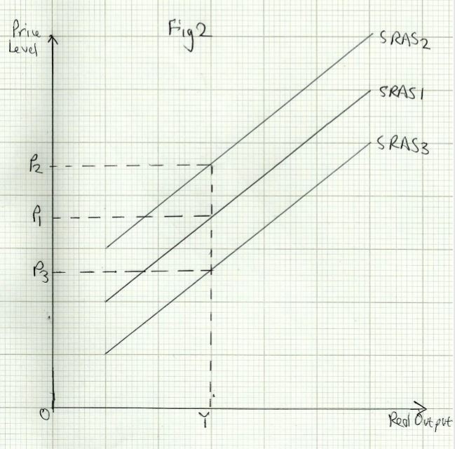
Shifts in SRAS are shown in Fig 2 above. Higher costs will cause the SRAS curve to shift upwards from SRAS1 to SRAS2 __(a decrease). Lower costs will result in a downwards shift from __SRAS1 to SRAS3 __(an increase). The same level of output at __Y could be associated with 3 different price levels, P1,P2 __or __P3, depending on the level of costs in the economy.

Shifts in LRAS

Over time, the LRAS is likely to move out to the right, as the capacity (or potential output) of the economy increases. This also means the production possibility frontier has shifted outwards. It can be described as a movement along the growth path.This is what economists call long run economic growth. An increase in LRAS can result from any of the following:

1. Technological change_ –_ Faster, more reliable machines can lead to higher productivity. __Automation __(replacing workers with machines) is the extreme example
2. Improving skills and education_ –_ This enables workers to move from low skilled, low productivity jobs to high skilled, high productivity work
3. Demographic change – The size of the labour force may grow through a higher birth rate, immigration or higher participation rate
4. Improvements in governance and institutions – Some countries suffer from high levels of corruption and mismanagement. They may not have a legal system that encourages investment. In some countries many industries are run as monopolies, making big profits for the owners (often the politicians), which discourages competition and efficiency

Note that it is possible for LRAS to decrease (move to the left) as well. Warfare, disease or natural disasters are some of the possible reasons.

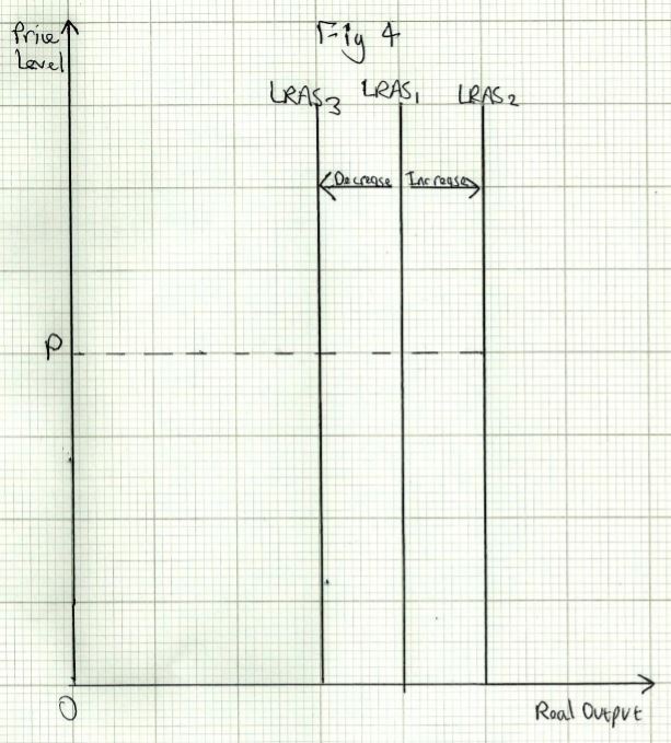
Shifts of the LRAS are shown in _Fig 4 (above). _An increase in LRAS is shown by a move to the right, from LRAS1 __to __LRAS2. A decrease is shown by a move to the left to LRAS3. Any given price level, such as P, can therefore be associated with different levels of output.

The Keynesian View

Keynes did not believe that the economy would always quickly adjust to shocks and return to the full employment level of output. He argued that it was possible for the economy to get ‘stuck’ at an output well below capacity, as it did during the Great Depression of the 1930s. Keynes believed that the LRAS was as shown in _Fig 5 _below:

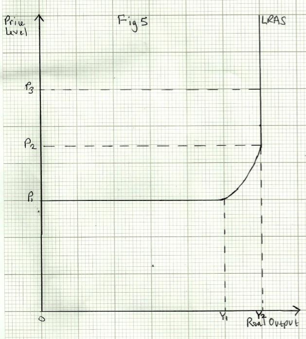
At output below Y1 __there is a lot of spare capacity in the economy (high unemployment). Keynes believed that in such circumstances the LRAS was __perfectly elastic: output could be increased easily without any upward pressure on prices (shown at P1). With high unemployment, workers would be in a weak position to demand pay increases. Equally, Keynes argued that it would be hard for the price level to fall below P1. This is because trade unions would resist wage cuts, and also because of minimum wage laws. Benefits also provide a kind of ‘floor’ to the wage level, as workers will not seek jobs if they are better off on benefits. If wages don’t fall, it is hard for firms to cut prices.

Between outputs Y1 __and __Y2, the economy is getting closer to its maximum capacity. Unemployment is much lower, and there may start to be a shortage of materials and factory space to rent. Factor prices will therefore start to rise. This means that beyond Y1, the price level will start to rise.

At Y2 the economy is at full employment and is perfectly inelastic. It is vertical, like the neo-classical LRAS. A short term increase in output is possible, but in the long run output will fall back to Y2, but the price level will be even higher (i.e. at P3).

The LRAS can shift to the right or left, just as with the neo-classical LRAS. This is shown in Fig 6 below:

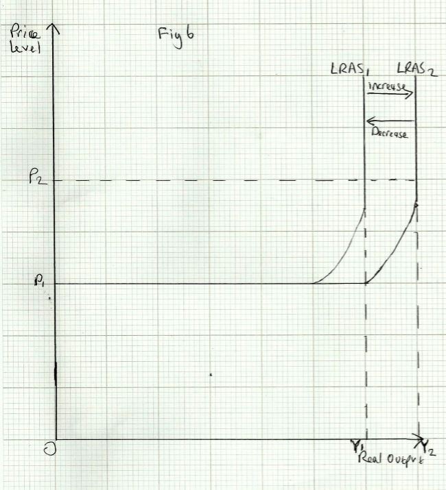
Any given level of prices (such as P2) can therefore be associated with different levels of output, (i.e. Y1 or Y2) as the capacity of the economy changes.

Long Run Aggregate Supply

Economists are divided in their views on the nature of LRAS, between the neo-classical view and the Keynesian view.

The Neo-Classical View

Neo-classical economists believe in the power of the free market to adjust to shocks and move back towards equilibrium quickly. For instance, if the economy is in recession, and there are unemployed workers and other resources, wages and other factor prices (ie. factory rents) will fall, as they are in excess supply. As they fall in price, demand for labour and other factors will rise. The unemployment is therefore self-correcting.

In the long run, therefore, the neo-classical view is that the economy operates at its full employment level of output. Put another way, it means it is operating at its maximum capacity. In other words, in the long run the economy is operating along its production possibility frontier (PPF).

The LRAS ‘curve’, on this view is a vertical straight line, at the full employment level of output, as shown in _Fig 3 _below:

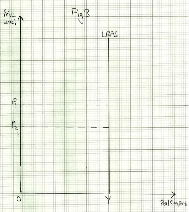
The economy is at full employment at a level of output shown by Y. Although it is possible in the short run for output to be higher or lower than Y, this is the level of output that the economy will return to, unless there is a shift in the LRAS. At all price levels (i.e. P1 or P2), the level of real output is the same.

If the actual level of output is above or below Y, there is an output gap.