Linear Functions with Graphs
Interpreting gradients
Key points when interpreting gradients:
- Steepness; the larger the number, the steeper the gradient.
- Zero Gradients. Remember for the equation y=3, the gradient =0 (i.e. a line parallel with the x axis).
- Negative and positive gradients, look at the direction of the slope.
Interpreting results of graphs in financial contexts
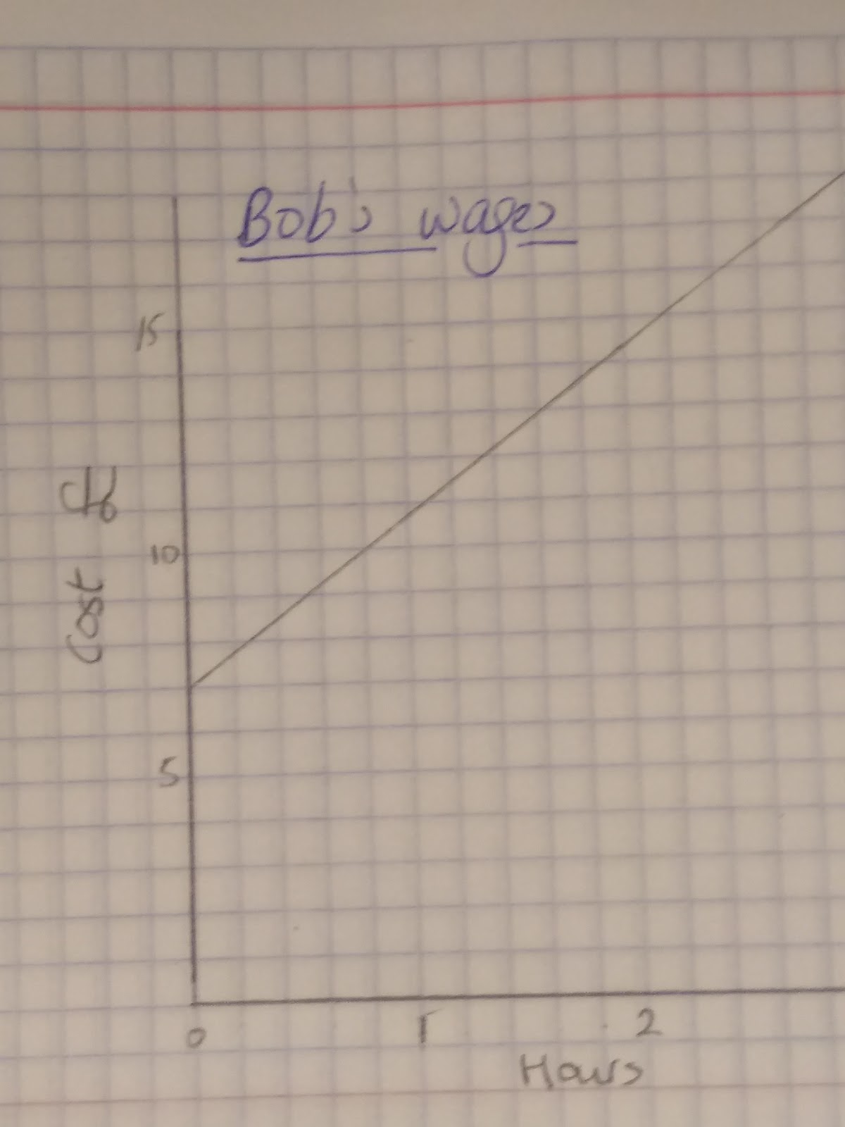
When it comes to real life graphs the gradient shows the rate of change. This graph shows Bob’s wages.
- We can see that the more hours he works the more he earns, however he gets paid the same amount per hour as the gradient does not change.
- The fact that the graph starts at £7 and not £0 shows us that he has a separate, initial charge of £7 before he has done any work at all.
- Also, we can see that this graph does not __show direct proportion__ because it does not go through (0,0). Think carefully about the information you can gain from the gradient and the y intercept. If the graph does not go through zero, think why this might be!
Interpreting results of distance-time graphs
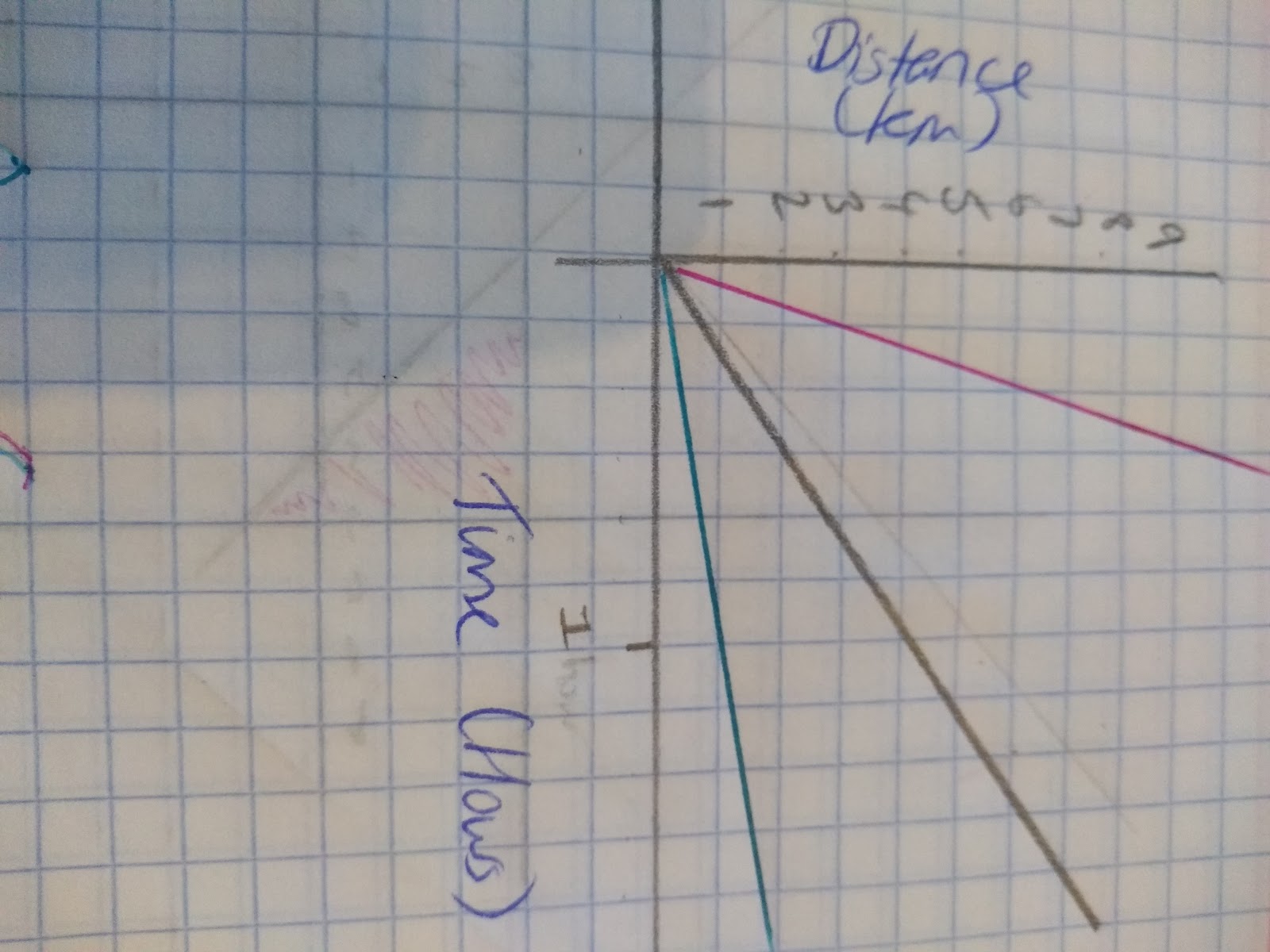
The gradient of this graph shows the speed. The steeper the gradient the faster the speed, in the graph above the pink line has the steepest gradient and therefore shows the fastest speed. The pencil is in the middle and the blue line is the slowest. In this distance time graph you can see that the gradient changes, and therefore the speed changes. This is a graph of someone running.
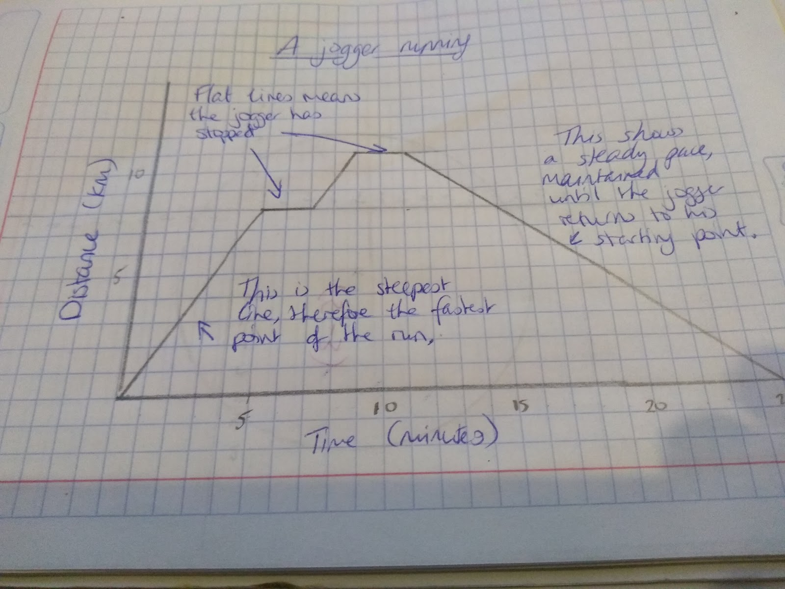
- When the gradient is flat that means that there is no movement.
- From the gradient we can see that the speed=0. This is the case from when the distance reaches 8km.
- We can also see that when the gradient is steeper, the person is moving faster.
- Remember on a distance time graph if the line returns to zero that represents the direction of the runner, they are going back to their original starting point.
Interpreting results of velocity-time graphs
The gradient on a velocity-time graphs show acceleration. If there is no acceleration the gradient will be zero, the speed will not be increasing or decreasing.
Velocity-time graphs are similar to speed time graphs in that the area under the graph is the distance. We can calculate this by working out the area underneath the graph.
In both graphs if the gradient is negative it means that the object is decelerating.
In the exam you may be asked to describe a velocity time graph. Here are some key things to include:
- The gradient at a certain point will give you the value of the acceleration
- If the line is flat (i.e. gradient is zero), that means the speed is constant (i.e. the acceleration is zero)
- If the line is going back towards the x axis (i.e. negative gradient) that means the object is decelerating.(i.e. negative acceleration).
Let’s describe this velocity-time graph:
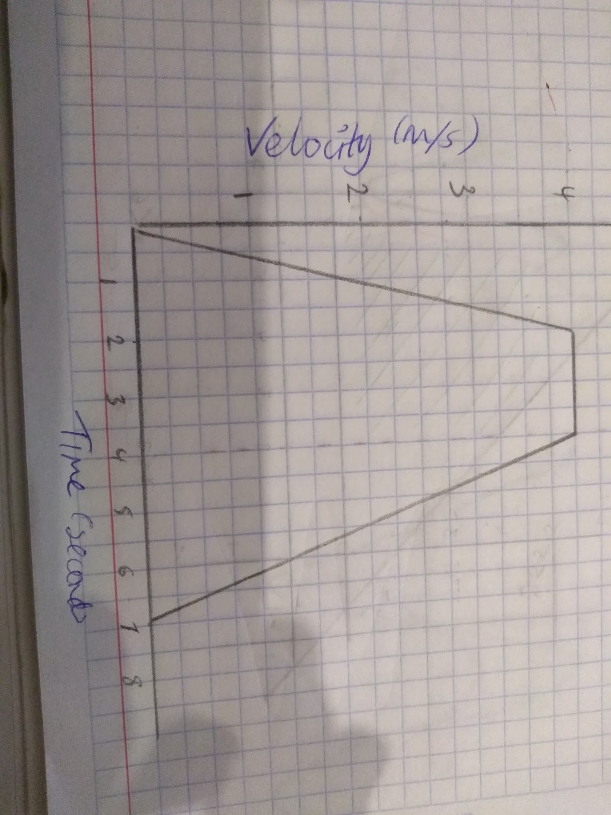
- Between 0 and 2 seconds:
- The acceleration is at 2m per second
- The object has travelled 4 m
- Between 2 and 4 seconds:
- The object is moving at a speed of 4m/s
- The object has travelled 8 m
- Between 4 and 7 seconds:
- The object is decelerating and is travelling at a speed of 1 ⅓ m/s
- The object has travelled 6m
Break down your graph into parts and analyse each for its acceleration / deceleration and the distance that the object has travelled.
- Which graph is steeper: a) y=3x +5 or b) y=-10x -6
- A is steeper
- The equation of a line is y=5x +9 , this equation represents the pay per hour of a science tutor. What can facts can you find from this linear function?
- That the intuition has a baseline fee of £9 and that they get paid £5 pounds per hour
- By drawing graphs solve the simultaneous equation y= 2x+1 and y=x+3
- Your answer should include: (2 / 5)